All About ANN – Artificial Neural Networks and Chemometric Modeling for NIR Spectroscopy

Artificial Neural Networks (ANN) are nonlinear models used in chemometrics that simulate the functioning of the neural network of human brains. Combined with Partial Least Square Regression models scores, these are used for machine learning and have important applications in many major industries and sectors, including food production.

Chemometrics for Near-Infrared Spectroscopy

The near-infrared spectrum is the solar radiation band commonly used to classify compounds found in plants and animals. It is also used to quantify the concentrations of components through spectroscopy.

That is because all living matter is made up of organic compounds that contain carbon (C), hydrogen (H), and oxygen (O). NIR spectroscopy is useful to measure organic compounds, as it interacts with chemical bonds between the basic elements: H-C, H-O, and H-N. Each compound will interact with a specific wavelength of NIR to absorb, transmit, and reflect them in varying amounts. So, the spectra produced by the compounds will vary; this variation is used to measure the difference in composition in fruits and judge its level of sugars and dry matter.

Common Predictive Models

However, the spectral data produced are complex and vast. NIR spectroscopy’s wide application in food science instruments is possible because the chemical data can be analyzed by a multidisciplinary science called chemometrics that combines statistics, software, and electronics.

Chemometrics uses multivariate statistical models to analyze the wide range of the spectrum, concentrations, or sensory characteristics of food samples. It is then necessary to choose the correct model to develop a tool with good predictive powers.

One of the factors influencing model choice is the type of data.

Models for Linear and Nonlinear Data

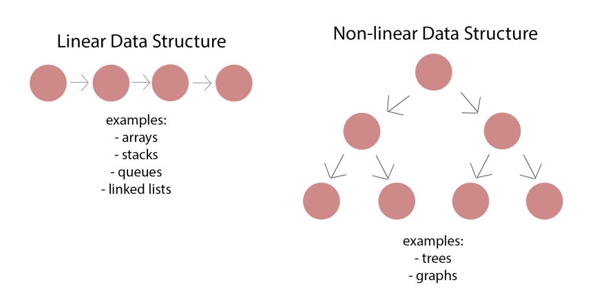
Figure 1. A diagram to show differences between linear and nonlinear data, Megan 2019. (Image credits: https://dev.to/mwong068/introduction-to-linked-lists-in-ruby-kgi)

The most common models that are used in chemometrics are Partial Least Square Regression (PLS), for quantitative chemometrics, and Principal Component Analysis, (PCA) for qualitative analysis of near-infrared (NIR) spectra.

However, these methods are most useful to analyze multivariate data when the relationship between the predictors (X) and responses (Y) is linear. Examples of linear data are stacks or linked lists, as shown in Figure 1. Here, the relationship between the predictor and the response is direct, and the equation for the straight-line graph is obtained by addition:

Y = bo + b1X1 + b2X2 + … + bkXk

Nonlinear NIR Data

When the predictor influences the response indirectly, nonlinear data is produced. When plotted, the graph produces curves of various forms. Graphs and trees are usually used to depict non-linear data; see Figure 1.

Curvature can be introduced in a linear model by using a squared variable, but the equation is the same.

Y = (B1 + B2*x + B3*x^2 + B4*x^3) / (1 + B5*x + B6*x^2 + B7*x^3)

If the algorithm does not account properly for nonlinearity in data, it can give the wrong model that will have low predictive powers, as shown in Figure 2 (a). In this case, a nonlinear model explains the relationship between X and Y more efficiently.

Both linear and nonlinear data have their uses. For example, linear data is used in software, while non-linearity is more useful in artificial intelligence and machine learning. This is because the hierarchical nature of non-linear data uses memory more efficiently and makes more sense of each data point.

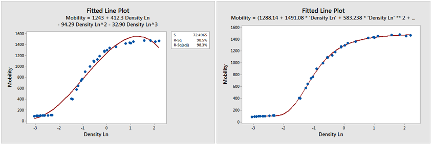
Figure 2 (a) and (b): Non-linear data is fitted with (a) a linear model and (b) a non-linear model; the latter explains the mobility of electrons better, Frost, J. (Image credits: https://statisticsbyjim.com/regression/choose-linear-nonlinear-regression/ )

PLS Models

Many NIR tools are mostly concerned with measuring concentrations of compounds for quality control during harvest and post-harvest and during processing. While PCA can be useful in some cases, it is PLS models used in quantitative measurements that get the maximum attention in the industry.

The basics of PLS need to be known in order to find out how the model is used to measure nonlinearity.

Multivariate linear PLS models use two blocks of variables, X (predictors) and Y (response), that are linearly related to each other; for example, between the X set, or NIR spectra, and the Y set, which could be concentrations of compounds or physical properties in a fruit. The model uses the covariance or relationship between the predictors and responses (for example, levels of concentrations that will influence the spectra).

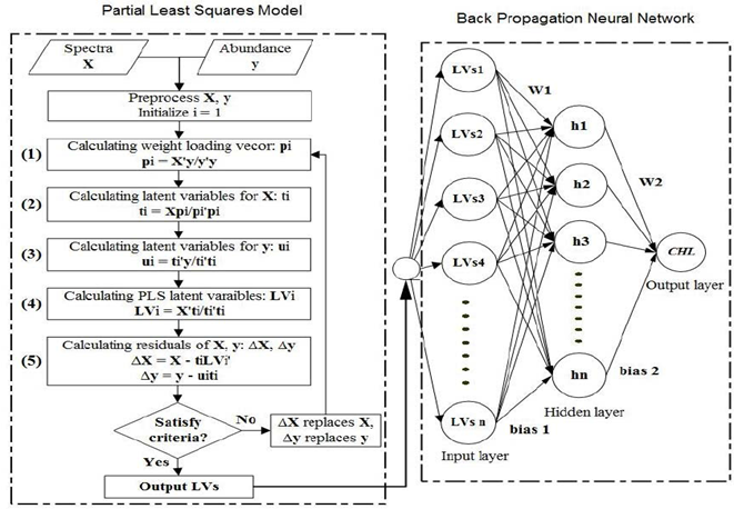
Figure 3: “Flowchart for PLS-ANN model. The PLS model shows the spectra processing for latent variables determination (left), and the BPNN shows how latent variables coming from PLS are processed by the ANN model,” Song, et al. 2014. (Image credits: DOI: 10.1109/TGRS.2013.2251888. )

PLS models aim to predict values of Y for future samples by identifying regression in the training sample set through the following steps:

1. Identify loading eigenvectors pi that explains variation in the X blocks, as shown in step 1 in Figure 3.
2. PLS then plots these vectors to get scores or latent variables through several iterations, where 1 explains the most variation in the Y set and t1 explains the most variation in response set X, as shown in steps 2 and 3 of Figure 3.
3. The PLS then plots the latent variables to get a score plot, which shows the regression or relationship (LVi) between X (spectra) and Y (concentrations), as shown in in step 4.
4. Iterations replacing X and Y variables with residuals from the previous iteration are used to get the latent variables in steps 2 and 3. In PLS Type 1, only one Y variable is predicted. In Type II PLS, more than one variable of Y or a block is predicted but is usually not as accurate as Type I.

A simple explanation of PLS is available in a video by XLSTAT.

Nonlinear Models

Many relationships between compound concentrations and spectra in plant and animal samples are nonlinear.

To account for nonlinearity, programmers are diversifying the models they use in chemometrics. The linear PLS models are adapted or combined with other models to tackle nonlinearity by taking two broad approaches:

• Adding Nonlinear terms
• Neural Networks

Adding Nonlinear Terms

One of the simplest methods used to account for nonlinearity in data is to introduce a nonlinear term in the linear PLS algorithm, as explained above. The nonlinear factor could be a squared x 2i, cubic x 3i, or higher-order polynomial term.

Without knowing the degree of nonlinearity—mild, moderate, or strong—data cannot be pretreated.

There are several methods to include nonlinear terms to produce nonlinear PLS models. These include Implicit Nonlinear PLS, Linear Quadratic PLS, GIFI Method, Polynomial PLS, Spline PLS, and Quadratic PLS. We look at two of the most common methods below:

• Implicit Nonlinear PLS modeling (INRL), where a squared term can be introduced to PLS. However, this increases the number of variables, making computation very difficult. Also, INRL cannot handle extreme nonlinearity, and their predictive power is close to those of linear models. An advantage of INRL is that it can identify outliers better than neural networks.
• GIFI method is also used when the nonlinearity is mild and for quantitative structure-activity relationship (QSAR) modeling. The variables are “binned” by dividing them by intervals into categories. These categories are now regarded as the new qualitative variables x1, x2, x3, etc. Each variable is assigned to all the bins, with a value of “1” if it falls within that range or “0” if it doesn’t. For an example, see Table 1. The new variable matrix is then used in Type I PLS. Binning can become time-consuming in vast data sets.

Table 1: Create intervals that become the new variables (x1, x2, x3) and bin the original variable in the column it belongs with a value of 1 and zero in the others.

Neural Network Models

The electrical activity of neurons in brains and the nervous systems have inspired a method called neural network (NN), which is a nonlinear model increasingly being used in chemometrics of NIR spectra.

Artificial Neural Network Definition

The Artificial Neural Network (ANN) is defined as a model that simulates a biological neural system, using a reduced set of concepts.

ANN or NN are trying to mimic the way a brain works to process data, which is far superior to linear computer computations. The aim is to produce algorithms or artificial intelligence that can process vast amounts of data in a very short time. Using ANN, accurate predictive models have been produced and are applied in a wide range of applications.

How does a neural network work?

Figure 4: “Sample artificial neural network architecture,” Walczak and Cerpa, 2003. (Image credits: http://www.sciencedirect.com/science/article/pii/B0122274105008371)

In a neural network, the calculation nodes (neurodes) are arranged in layers or vectors. When the signal from a predictor variable (x) reaches a node, it is processed and the output is sent to all nodes in the next layer. The processing performed by each node in is a calculation that could be linear or nonlinear and is also called the activation function. The output is passed with a coefficient (or weightage), wn,m, given to each activation based on connection.

The end output is a summation of y = Σwijxi

During the training of the model with data, the coefficient is adjusted as the model is calibrated or learns to correctly predict the known response from an input variable.

Activation function refers to whether the neuron is going to be active or not. If the output to the next neuron layer is 0, that activation is “off.”  The calculation that gives correct results is given more weightage as calibration/learning proceeds. The ANN learning adjusts the weight to connections between neurodes. The higher the weight given to a connection, the stronger the impact of the input with which it is associated. This way, correct calculations are chosen over incorrect or less accurate ones.

To calibrate the model, training data that include input variables with known responses or outputs are used.

An ANN structure has an input layer, an output layer, and one or more hidden layers in between. For example, there are two hidden layers in Figure 4.

ANN modeling has several advantages:

• It is a nonlinear computational tool
• It can find a functional relationship between input (predictor) and output (response) variables
• It does not require the development of an explicit model
• Failure of one element does not affect the efficiency of the system, as there are many nodes in a layer

Despite the advantanges, ANN models also have disadvantages:

• Large ANN models can have longer modelling times, however prediction speeds are comparable.
• Until recently, it has not been possible to explicitly identify the relationship between predictors and response sets. This can now be achieved via permutation of variables.
• Requires larger data sets than conventional models (PLS)

PLS-ANN

Combining ANN with PLS can give better results than using either of the models alone. The latent variable matrix (LV) created by PLS can be used as the input for ANN, as shown in Figure 3 B. For spectrometers that utilize high numbers of wavelengths for inputs, use of LV scores can decrease model development time.

Two types of ANN are used in chemometrics:

• Multilayer feed-forward neural networks (MLFs)
• Supervised modifications of Kohonen self-organizing maps (SOMs)

Artificial Neural Network Examples

ANN machine learning is used in many industries, including food, pharmacology, finance, and industry, for:

• Pattern recognition
• Quality Control
• Processing

ANN has been tested and has been found to give accurate results in several parts of the food supply chain. Therefore, it is being used increasingly for modeling in food engineering.

• Pattern recognition gives input data a label based on machine learning; the most common use is face recognition software. In the food industry, ANN machine learning is used to classify different varieties of food, including

-Identifying types of beer

-Differentiating the ripening stages in fruits, such as bananas, based on phenolic content

-Processing of remote images for precision and smart farming

• Food quality control uses ANN models for prediction to perform several tasks. Some applications that have already been tested include the following:

-Judge firmness in kiwis

-Determine color in apples

-Detect spoilage by spotting bacterial growth in vegetables

-Authentication of food by tracing its geographical origin

-Find nutrients and predict antioxidant properties of spices (cinnamon, clove), pulses (mung bean, red bean), cereals (red, brown, or black rice), and beverages (tea)

• Processing of food typically needs multilayer ANN to find the best conditions to get the desired result. For example, in the case of bed drying of carrots, an ANN model was used to find the energy use needed for different combinations of drying time and air temperature, carrot size, and bed depth.

Data-Driven Agriculture Needs ANN Modeling

As the role of biochemical data in agriculture increases in every stage of the supply chain, a means to quickly and accurately analyze the data and get actionable insights from them is needed. ANN offers a means to analyze multivariate data with indirect relationships, which is more the norm than the exception in the natural world. Starting from advising farm operations to quality control and food processing, ANN models in chemometrics hold the key to produce food that is safe for people and the environment.

—

Vijayalaxmi Kinhal
Science Writer, CID Bio-Science
Ph.D. Ecology and Environmental Science, B.Sc Agriculture

Feature photo courtesy of Moritz Kindler

Sources

Bedford, S. (n.d.). Machine Learning & Food Classification. Retrieved from https://simonb83.github.io/machine-learning-food-classification.html
Chemometrics. (n.d.). Retrieved from http://ww2.chemistry.gatech.edu/class/6282/janata/Multivariate_Methods_Nutshell.pdf
Dearing, T. (n.d.). Fundamentals of Chemometrics and Modeling. Retrieved from https://depts.washington.edu/cpac/Activities/Meetings/documents/DearingFundamentalsofChemometrics
Difference between Linear and Non-linear Data Structures. (2020, April 22). Retrieved from https://www.geeksforgeeks.org/difference-between-linear-and-non-linear-data-structures/

Geladi, P., and Kowalski, B.R. (1986). Partial least-squares regression: a tutorial. Anal. Chim. Acta, 185, 1–17. DOI: https://doi.org/10.1016/0003-2670(86)80028-9

Guiné, R.P.F. (2019). The Use of Artificial Neural Networks (ANN) in Food Process Engineering. International Journal of Food Engineering, 5 (1). DOI: 10.18178/ijfe.5.1.15-21

Mörtsell, M., and Gulliksson, M. (2001). An overview of some non-linear techniques in Chemometrics. Retrieved from https://www.researchgate.net/profile/Marten_Gulliksson2/publication/237317769_An_overview_of_some_non-linear_techniques_in_Chemometrics/links/0046352cbdb17787dd000000/An-overview-of-some-non-linear-techniques-in-Chemometrics.pdf

Puig-Arnavata, M., & Bruno, J. C. (2015). Chapter 5 – Artificial Neural Networks for Thermochemical Conversion of Biomass. In (Eds) Pandey, A., Bhaskar, T., Stöcker, M., & Sukumaran, R.K. Recent Advances in Thermo-Chemical Conversion of Biomass, Recent Advances in Thermo-Chemical Conversion of Biomass. Elsevier, 133-156. ISBN 9780444632890. https://doi.org/10.1016/B978-0-444-63289-0.00005-3.

Scholz, M. (n.d.). Nonlinear PCA – Nonlinear PCA toolbox for MATLAB. Retrieved from http://www.nlpca.org/

Song, K., Li, L., Li, S. et al. (2014). Using Partial Least Squares-Artificial Neural Network for Inversion of Inland Water Chlorophyll-a. in IEEE Transactions on Geoscience and Remote Sensing, 52 ( 2), 1502-1517, doi: 10.1109/TGRS.2013.2251888.

Svozil, D., Kvasnicka, V., and Pospichal, J. (1997). Chemometrics and intelligent laboratory systems Tutorial Introduction to multi-layer feed-forward neural networks. Chemometr. Intell. Lab. Syst, 39(1), 43–62.

Walczaka, S., & Cerpab, N. (2003). Artificial Neural Networks. In (Ed.) Robert A. Meyers, Encyclopedia of Physical Science and Technology. Academic Press, Pages 631-645, ISBN 9780122274107,
https://doi.org/10.1016/B0-12-227410-5/00837-1

Workman, J., & Mark, H. (2020, Aug 1). A Survey of Chemometric Methods Used in Spectroscopy. Spectroscopy, 35(8), 9–14. Retrieved from https://www.spectroscopyonline.com/view/a-survey-of-chemometric-methods-used-in-spectroscopy

Zareef, M., Chen, Q., Hassan, M.M. et al. (2020). An Overview on the Applications of Typical Non-linear Algorithms Coupled With NIR Spectroscopy in Food Analysis. Food Eng Rev 12, 173–190. https://doi.org/10.1007/s12393-020-09210-7