Welcome to the third installment of our Future Proof Your Quality Webinar Series!
In this episode, our esteemed Director of Applied Science, Galen George, guides us through the detailed steps of building a model, including pre-processing, various types of Near-Infrared Spectroscopy (NIRS) models, and wavelength selection.
This webinar aims to deliver comprehensive insights on spectroscopy in commercial agriculture, focusing specifically on internal quality assessment and chemometrics. Galen’s presentation is designed to accommodate beginners and experienced professionals in the field.
In this episode, you’ll learn about:
1. Pre-processing techniques such as Mean-centering, Standard Normal Variate (SNV), Savitzky-Golay (SAVGOL) smoothing, and Derivatives.
2. Various types of models, such as Principal Component Analysis (PCA), Partial Least Squares (PLS), and Artificial Neural Networks (ANN).
3. The advantages and considerations of choosing between a broad wavelength range and targeted wavelength selection in model building.
A Live Q&A was hosted following the webinar.
This series has received rave reviews from our agriculture partners, providing valuable insights into the future of tech in the field of agriculture.
Don’t forget to stay connected for the release announcement of the fourth episode of our series. If you haven’t done so yet, consider subscribing to our channel and hitting the notification bell, so you won’t miss any future webinars. Your support helps us create more high-quality content related to the future of agriculture and technology.
For any questions or comments, please feel free to leave them in the comment section below. We appreciate your feedback and will do our best to respond to each.
Thank you for watching, and we look forward to seeing you at our next webinar!
Full Transcription
It is time to start our webinar welcome everyone and thank you for
coming today this is the third webinar in our six-part series
about practical chemometrics and the agriculture sector um today’s webinar is going to be our
second part of our building a model a portion of the webinar series and today
we’ll be talking about pre-processing types of models and wavelength selection
before we move on I want to get through some light housekeeping oh
just a couple slides there first my name is Galen I am the director
of applied science here at Felix instruments I’ve been with the company for four years now my background is in
Biochemistry and food science and previously worked in uh quality and
safety testing in the agriculture food and cannabis sectors
also joining us today is Susie Truitt our distribution manager she is uh um
basically being the admin of the uh whole meeting and so she’s actually
going to be the one in the chat uh posting any relevant links she’ll also be directing you towards uh
any other resources that we might uh as far as questions that you might have
um that we can’t address today um so please if you are uh interested in
asking a question do not use the chat function please use the Q a function in
Zoom that way I can see it at the end of the webinar um if you do post a question in the chat
there’s a chance I might not see it we might not get to answering it if there are any technical issues if suddenly I
disappear or you can’t hear me anymore or the call drops something like that please put that in the chat uh so we can
address that before I keep rambling on without anyone actually being able to hear me
uh so without further Ado let’s go ahead and just jump into a little bit of a review so
well we’ve talked about thus far and it’s been a little while but what we’ve talked about thus far uh in the model
building process is sampling and collecting the Spectra and Performing
the analytical testing necessary to actually have the data build the data sets out to actually then build a model
with so we’re at the stage now where we need to start using our multivariate data
analysis our chemometrics to actually take this data and build it into a
predictive model or a discriminant model depending on what the application is and
so that’s what we’re going to be discussing today the next stage is going to be the model deployment and before we
even deploy model we also need to validate so that’s what we’ll be talking about next in this process
um but just a little bit of a uh review on what we talked about last time
and this is important for today because as much as what we talk about today does
matter and has an impact in the quality of the models you build the most important part and I think many
people would agree with this the more important part of this this process is in the sampling and the testing and this
collection of the Spectra because the saying is garbage and garbage out so if
you have bad data in your model you’re gonna not ever have a really well-performing model it’ll be a bad model
and so really it’s all about having high quality data going in to the model
building process and then this stage that we’re going to talk about today is kind of just a little bit of the icing
on the cake it does have an impact but it’s not nearly as significant of an
impact as the quality of the data in the model so that is definitely the more important step today there is a lot of
information what we’re going to do is give you the 30,000-foot view so just
the kind of overview we’re not going to get into the mathematics of all these different techniques
um just going to give you an idea of what’s out there what’s been used in the past what is currently being used and
then we’ll talk about some use cases and then we’ll just talk about the practical application of all this information
so multivariate data analysis or chemometrics coupled with nir
spectroscopy really has three main steps so we have a Spectra pre-processing
wavelength selection step and then a model selection so just choosing what kind of actual modeling method we’re
going to use and within these three main categories of steps we also have dozens and dozens
of different methodologies that have been developed and utilized in Academia and research in practice and so we’re
not going to be able to get to every single one I’m going to talk about some of the more common ones we do have I do
have some literature that you can some amazing reviews actually that you can uh
take a look at yourself in your free time if you want to learn a little bit more in-depth about these processes
so first in this pyramid that you just saw we’re kind of going to build from the first step which is the Spectra
pre-processing then we’re going to build to the next step which is going to be our wavelength selection and then our
last step which is choosing which model to use so I’ll start by talking about all a bunch of different pre-treatment or pre-processing methods
uh and so off the bat there’s gonna be a million
you’ll see a million different uh variations of these methods so even
Within These methods, there are absolutely different methods methodologies Within These methodologies
uh and so there’s that’s where I’m bringing up there’s just so many out there it’s hard to know what to actually
choose or use but these are just the kind of overarching types of pre-processing
um so the first one is spectra smoothing and this is the most common uh step that you’ll see uh when you’re ever you’re
building models and this is just as this picture denotes this is really just taking all of that little bit of extra
signal to noise all that little bit of noise and smoothing it out so that you’re not accidentally creating
correlations with something that isn’t actually useful information and so uh this is usually the first
pre-processing step for most models um but like I said it’s almost always
just a first step it’s always used in a
tandem with another pre-processing or pre-treatment method
um another uh common pre-treatment method uh is just to adjust the Baseline
drift with an offset correction so if you have a consistent uh um bias in your uh in your in your
Baseline of your Spectra then it’s pretty common just to take back and shift it down so that it’s All Uniform
across all of your data um another similarly to that uh
sometimes it can be seen that there’s an actual uh linear Trend in the Baseline drift so instead of just a constant uh
kind of offset in your drift you actually have a a changing a gradually changing drift and so for that they just
call it D trending but really what you’re doing is just fitting a least squares trend line uh to your Spectra
and then subtracting that from the original Spectrum so that it kind of centers everything back down to uh being
on the same Baseline like I said so these first three that I just mentioned
almost all used in tandem with other methods so it’s just like the initial first step just to kind of get your
Spectra in a in a kind of standardized way right there’s also like mean centering and other methods similar to
this that uh that do similar things where we’re just taking try to get all of our Spectra onto the same kind of
scale and the same uh Baseline get it all smoothed out before we actually then
go and do some of these other methods so uh two of the other most common uh
methods that you’ll see after you’ve done these other uh smoothing or Baseline Corrections is multiplicative
pattern correction or MSC um this is pretty commonly used in a lot of literature
um really what this method as well as standard normal variate or SNB they’re
both pretty much accomplishing the same thing just using different methodologies to do it but really what they’re doing
is trying to compensate for uh non-uniform scattering non-uniform particle size
um and so taking uh that and and trying to actually uh reduce any kind of uh use
non-useful information get it all kind of uniform all the special uh uniform
um and so they just do it using different methods of typically some some combination of uh taking the average of
the Spectra and uh dividing that by the same deviation and then subtracting that
from the original or other kind of variations of of that kind of methodology
um as far as another one other really common uh addition to the pre-treatment
process is the derivatives so the raw absorbent Spectra
um isn’t always necessarily the best type of Spectra to use and so after you’ve
done smoothing a lot of the times what you’ll see are people taking first or second derivatives uh this also helps
with uh eliminating drift or scattering um non-uniform scattering as well
um so the second derivative Spectra is a pretty common uh pre-treatment that
you’ll see some people like to use their absorbance uh as well and but really uh it just
comes down to in practice what is going to be most practical for you and what gives you the best performing model
as far as kind of newer and not as well studied or used methods for
pre-processing we have things like wavelet transformation orthogonal signal
correction and net analyte pre-processing um so all of these things help with very
specific kind of problems within your within your spectral data set
um and so wavelet transformation is more a data compression technique
um orthogonal signal correction helps a lot with outlier detection and calibration transfer uh and then net
analyte pre-processing that actually is more of a uh when you have a mixture but
still fairly uh finite mixture not a usually not typically a living uh kind
of uh or you know a biological system usually more of a chemical mixture and it helps with separating out and
individual analytes or ingredients within that mixture so those are more for like very specific things if you
know if you go into a an application you know where you are trying to build a model and you know that you’re trying to
accomplish a specific task like separating ingredients out of a mixture or uh you know you want to deploy a
model across a bunch of different types of instruments a bench top uh nir a
handheld nir in a whole bunch of different models then you’re going to want to maybe think about orthogonal
signal correction um as to help out with that calibration transfer across devices
um as far as you know which are most common and which are used the best are which are which are methods just are are
the best methods to use it’s going to be application specific every single time and so really you just have to look at
your data set and figure out on your own what things you need to do to get that
data set as smooth and kind of uniform as possible while still retaining the
important information that you need to get out of that Specter which is going to be you know where things are
absorbing in the wavelength range and being able to see Peaks and valleys within your Spectra
so it’s really going to be up to you uh to decide that we’ll go into more details about that here later but I want
to get through um the actual methods first and then we’ll talk about some practical uh
aspects of this so the next uh
section or step in the process right is wavelength selection uh here there’s a number of different
ways to go about it as well a whole bunch of different methods uh you’ll see that there are these are all basically
essentially ways of figuring out in the entire wavelength range that my
instrument uses which wavelengths are giving me the most important information
so there’s a number of kind of basic ways to do this and then more and then as the years have gone on we have more
and more complex algorithms to help us determine which wavelengths are going to give us the most valuable information
for this model uh and so Spa successive projections
algorithm that’s a pretty commonly used uh uh algorithm that uh you’ll see in a
lot of literature that one as well as regression coefficient which is just the most basic
way of determining your wavelength importance is by just looking at
according to my plsr model that I just built which wavelengths are given the
highest absolute values in their coefficients and so that’s just like a very basic uh
way of doing it loading weights is a very similar to regression coefficient you’re just using the loading weight
instead of the um the absolute value of the coefficient and then you have stuff like genetic
algorithm which is a iterative process where it’s basically starting off with
one wavelength and then it’s adding on a new wavelength depending on how often that wavelength was utilized in all the
other iterations and prioritizes all these wavelengths based on this iterative process that uses a fitness
function which is essentially just saying that every anytime the rmse of
cross-validation which is the root mean square error of cross-validation is is
the lowest then that means that that was a good model so we’re going to keep that
wavelength and then we’re going to and prioritize a new way of life and see how well that model gets built how low that
RMS ECB is and we’re gonna so then it just prioritizes wavelengths in Us in that kind of way
um competitive adaptive related sampling um essentially the same as uh the
regression coefficient method um but then you also uh create subsets
from those essentially from those uh regression coefficient uh methods that you used
create subsets of variables and then you do the same kind of iterative process to
figure out which models give you the lowest rmsecb uh uninformative variables elimination
this is kind of an interesting one um this is actually uh different than most of the other ones because you’re
actually adding in variables that are just noise
and then you’re building a model you’re calibrate you’re building an actual model with those noise variables in it
and then you’re seeing which of the actual experimental variables that you
have are are as are essentially equivalent to the noise variable that
are equivalent to the noise variables and so when you can determine which experimental value variables are
equivalent to those noise variables that you artificially introduce then you know that those experimental variables have
no important information because they’re equivalent to the noise that you just added in and so you can just eliminate
those and whatever’s left is your variables that you want to select when I say variables I’m talking about
wavelengths uh so that’s just all kind of interchangeable terminology um and so uh these are all you know all
well studied and they’ve been used in literature and and academic studies
but when it comes down to it what we’re trying to do is with this is is Select
where the most important information is in our wavelength range from our instrument with the F750 we’re looking at mostly in
the nir range right we’re looking right from 700 to 1200 nanometers
and there’s some information there there’s some third overtone information about CH
bonds and NH bonds but really we’re dominated by the oh Bond we’re dominated
by water and for the most part in practice it is
almost always just it’s easier and it doesn’t really change performance that
much to just use the entire wavelength range so that’s either called full band or
it’s just called not doing wavelength selection um and so when you do full band
wavelength selection or no wavelength selection really you’re still getting all the
information you need but now you’re just relying on other parts of your model building process and you’re D and you’re
relying heavily on your data collection to make sure that you’re not getting all
these confounding variables or unimportant signals uh uh in your in
your data set that are going to cause your model to perform poorly and really this is uh in practice I
think what is used most commonly and so because it’s Simplicity because it
doesn’t require a whole bunch of data scientists in a room to to do all this kind of uh wavelength selection and it
doesn’t require rigorous you know studying um that it just seems like the most
practical way to go about things and it overall hasn’t really doesn’t really affect performance in the and and then
in a very negative way that you might think it would because all these wavelength selection uh methods exist
you might think oh it’s really important to do that but really it’s been shown many times that it’s just not that it’s
not as significant to the performance overall performance of the model as you
might think so those are the first two steps right
we’re pre-processing our Spectra and then we’re selecting wavelengths in many cases we’re just selecting the full
wavelength range of our instrument um and so or just the full wavelength
ring of range of the nir or just the full wavelength range of the visible light whatever it is that you’re trying to accomplish
um and so now we’re at the stage where we know we want to do these things uh I had it you know ahead of building the
model and then we want to now select which model type is going to be best for
us so I want to start with discriminant methods because this isn’t a super
common application as far as uh the Felix
instruments line of instruments is concerned but it is uh an important application in a lot of agricultural
sectors when you’re trying to do simple things such as detect bruising early
bruising or detect disease or detect rocks or or just even sorting quality
into a kind of qualitative uh bins where it’s you know low quality high quality
medium quality um and so these methods are important to explore because they they are do have a
usefulness um with this technology with an IR spectroscopy so uh PCA is kind of the
original uh just uh chemometric method for
um really what it’s used for mostly is a reducing the dimensionality of data
um and also and also looking for relationships looking for uh these kind of discriminant uh data sets where in a
larger data set can we see is there a difference between you know this this type of fruit this
unrodded fruit and this fruit that is rotted um but really it’s mostly used it’s not
ever really used on its own as a model building technique it’s more a used as a
precursor to then performing one of these other methodologies
um plsda which is partial D squares discriminant analysis
um this is probably one of the more common types of discriminant methods in the literature uh plsda is essentially
just a partially least squares regression model but instead of having
analyte quantities as your why Matrix variables you have just a dummy variable
like a one or a zero or something like that so you’re just or a one two and a
three it’s just a placeholder variable that establishes a a class for your for
your different um groupings of of samples and so that’s that’s essentially how
that method works for uh some other uh methods that are also used uh maybe not
as commonly but uh still uh used are the Simca method which is soft independent
modeling of class analogy um so this one uses PCA uh basically a
PCA model for each class uh in a certain training data set
um and then each observation is assigned to a class based on the residual distance from the model
um and so this is a just essentially a more a slightly more complicated PCA uh
method LDA linear discriminant analysis I would say I see this one
um this one and support Vector machine are probably the second most common to PLS VA linear discriminant analysis
um is uh good for both classification and data dimensionality reduction so just like PCA can reduce data
dimensionality LDA also works really well in that way support Vector machine is probably on
the newer side as far as all these other methods are concerned
um but uh this is a great method for when you have linear and non-linear data
so if uh um if you’re basically what you’re trying to study doesn’t have some
some sort of linear relationship with uh uh the Y Matrix which is the class
that you’re trying to study um then then this is a great method uh that you can use for that
but discriminant methods uh are definitely less common I would say and
and what we’re trying to do uh then the actual quantitative calibration methods
and so this is really the more uh important uh part of this that I wanted
to talk about um so there’s been a progression of what
kind of models are used the most in uh commercial agriculture when we’re
talking and agricultural research when we’re talking about nir spectroscopy so
this is it acts as kind of a timeline really and also in that way helps guide
us into what we kind of should be looking for when we’re choosing a a methodology
so it started off with multiple linear regression uh which is just a a very
basic linear regression kind of algorithm um but if you have multi-collinearity
between your variables then you’re not going to be able to use this methodology so if you have
variables that are uh similar to one another and they’re both increasing at
the same rate or and there’s you know it’s a complex system mlr isn’t going to work the best
in general I would consider most agricultural agricultural Commodities a complex system so this is not a
technique that I would really recommend anyone be using anymore because we have advanced so much further than this
the most common uh probably uh and I believe this is uh from uh a recent
review published by Carrie Walsh and Nick Anderson uh but plsr I think accounts for over 40 percent of
published papers on nir spectroscopy and uh commercial agriculture so plsr was uh
really used heavily throughout the 90s um because not only because uh you know
it was a you know the best of the time but also because it was widely uh
available in a lot of different software packages like Matlab and unscrambler and
and things like that so these statistical software packages um had the ability to run these plsr
models uh uh and so this became a very popular way to go about building models
um it’s just much easier to just plug your data into a uh a software and then
click a button and have it give you you know output a model
um from there we started to go into uh uh the least Square support Vector
machine um this one actually has a decent amount of Publications in recent years
um this is kind of I view it as more of a academic uh kind of situation where I
don’t I’ve never really seen this used much outside of Academia um so I think it’s just uh if you have
the ability to test it and see how well it performs versus other types of models sure it might be nice to try the least
Square support Vector machine from a practical standpoint I don’t really see the benefit because around the same time
we also started implementing artificial neural networks and artificial neural
networks are amazing for complex non-linear systems so essentially
anything that is a a commercially available uh you know Agricultural
Product is a complex system uh and it’s a you know it’s a living biological
system and there’s it’s not just you know three chemicals in a pile uh in a
powder form so it’s amazing at being able to generalize across all these
different uh you know seasonality regionality all these kind of issues and
variables that we talked about in the last webinar um artificial neural networks are are
great at kind of overcoming these obstacles and they’re especially useful when we have these large diverse data
sets so sure plsr might predict really well
if you are only looking at one variety of Apple grown in a single Orchard and
you’re using a single instrument and you only looked at it in one season yeah that model might be the best possible
model you can make plsr might outperform everything else but in practice if you wanted to then
use that model the next season you’re gonna run into some a lot of difficulties using that and it will not
be an accurate model however if you use something like an
artificial neural network and you put into practice the things that we
talked about last webinar things like collecting data across different instruments across multiple Seasons
regions whatever you need wherever you need the instrument to predict you
collect data from that variable and you include it in your data set the neural
network itself is highly capable of sussing out all these little kind of intricacies
within the data and seeing those relationships and being able to compensate for those things so
temperature changes in temperature if you just you know it’ll be able to see that you know as there are like there’s
a relationship here between this Spectra changing because of the temperature and
the actual bricks value so we’re going to compensate for these changes in the
Spectra and make sure that they’re not over predicting or under predicting during these changes in temperature
so artificial neural networks are really what are being uh utilized the most
right now uh typically in this in a commercial setting so when we all of the
Felix instruments uh models we use artificial neural networks um and it’s just a it’s a great tool for
for building in all this variability and being able to still get a robust well-predicting model across all these
all these variables that present challenges for this technology
now that being said we are now in an era where neural networks have actually been around for a
very long time we just finally started getting around to using them more often in the last 10 years
but now we’re in an era where Computing is uh computing power and Computing
algorithms are increasing exponentially every day and we’re finding that there’s
newer and newer deep learning techniques that could be even more beneficial to
this technology than the art the the the kind of Baseline artificial neural
network so there are other artificial neural network architectures that are deep learning
techniques that we can start to explore to actually see whether or not we can
get even better performance with the benefits of having to do you know
shorter training times when you’re actually building the model uh parameter reduction
um down sampling so basically reducing um all the the Computing load of of
these models but still getting the exact same performance which would mean we
could build you know where as whereas right now it might take us for a 10 000
sample set model it might take us four to six hours to build a model to train a
model now it might only take us an hour to train a model and so that allows us to
run even more iterations explore more options uh to ensure that this model is
the best performing model we could possibly put out so this is a Avenue that we’re going to be
starting to explore the convolutional neural network um essentially like I said it’s just a
different type of artificial neural network architecture um that it’s doing slightly different
things than a typical neural network is um but it’s uh really exciting and
there’s even more deep learning techniques that are available that we can start to explore now that we have uh
the resources to do so we have you know we have all these Cloud uh cloud-based
servers that have all this information already built into them and we can just start exploring and seeing you know how
well these models can perform with the convolutional neural network with other types of deep learning uh structures
so before I get into any formal recommendations uh for this kind of uh
you know this whole process of choosing Spectra pre-processing and and wavelength selection and model types
let’s first just look at two use cases and so I can kind of use those to to
help you understand how to choose all of these different between all these different
methodologies essentially so our first use case is going to be
uh a Chinese farmer that grows a single variety of jujube uh from a single
Orchard wants to build a model to non-destructively predict their soluble solids content
um so this is a quantitative predictive model and they only wanted to play it on a single instrument a single f750.
so uh they explored uh multiple different types of
wavelength selection methods they decided to utilize uh the multiplicative
scatter uh method of uh spectral pre-processing and then for their calibration methods
they wanted to look at both plsr and the LS svm
so uh looking at they you know every permutation of this combination uh are
of these uh various uh methods they tried every single permutation and uh
you know just examine their results to see which one is going to give them the best results so looking at the uh
methodology so they always used MSC for their pre-processing but looking at the one where they did no wavelength
selection or a full band selection essentially and I just used MSC for
pre-process and they used a plsr calibration method then actually gave them the best performance uh and uh you
know it’s it’s another one of those uh things where you can try you know you could put a lot
of work in and use all these different types of methods but it could turn out that the easiest the easiest and most
practical one is actually the best performing one and we see that actually a decent amount uh for instance what they’re using uh
here the MSC and then they used a stepwise regression analysis which is another wavelength selection method uh
and then they use plsr that gave them a 0.06 reduction in their r squared and uh
increase their error by 0.3 uh and for soluble solids that might be
you know 1.3 1.3 1.4 might be too high of an error average error to use in
practice for uh the MSC Spa uh the projections
algorithm and then uh using the ls svm calibration method gave them an even
worse r squared but the rmsc went down slightly um so it was just in between the two
methods now this is where I want you to see the kind of the bigger picture
what I said at the beginning the sampling is the most important part and that this is more like the icing on the
cake the you know just something you can experiment with but isn’t gonna determine the overall quality of the
model nearly as much as the sampling and the testing
here’s where you can see that evidence we’re talking about differences in the hundreds uh for most of these statistics
and you know this is a lot of work this is a lot of work to go through all of
these different wavelength selection methods and pre-processing methods and calibration methods they’re you know
they’re changing all these things around they’re trying every single permutation but in the end it’s only changing the
model just slightly you know very very slightly so it’s really you know it’s it’s
important to understand that in practice like this is it’s fine if you’re a researcher and you’re doing something uh
and you want to you want to cover all your bases you want to actually see evaluate the performance that’s you know
part of what you actually want to look at is all these different types of methodologies that’s great
and and you can absolutely do that but for for everyone else that’s
actually wanting to use these in practice um in their commercial operations
this is maybe not the most practical way to go about doing things and simplicity
is oftentimes just as high just as good as far as selecting these methods
Simplicity is just as good as going through and doing the super exhausting work of checking out every single
possible permutation of and combination of these methods
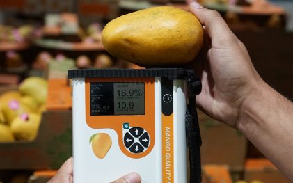
so let’s look at another use case this use case is in Australia and we
have a network of Australian mango Growers with dozens of orchards dozens
and dozens of orchards spread out across various regions across the entire country
uh and they want to create a model that will non-destructively predict dry matter and bricks in several different
mango varieties four you know four to six different mango varieties uh and they want ability to deploy this
this singular model on over 30 different devices and they want those devices to
be going out to all these different regions and taking measurements and they want them all predicting fairly similarly
so uh What uh what we’ve done or what they’ve done uh is uh do savitsky gole
smoothing and then svitzky gole second derivative
uh and so what we’ve done is smoothed out the Spectra done this gotten the second derivative of that Spectra
and then it’s time to choose the wavelength and they’re really just going full band uh essentially full band uh
nir so not really selecting any particular wavelengths uh not doing any uh not
performing any algorithms or methods to select specific wavelengths um and then for the calibration method
using a neural network and collecting good data from all these different
regions from all these different varieties across multiple different instruments calibrating them using the neural
network they’re getting an RMS EP of on average
less than one so this is an RM SCP which is on an
independent validation sense that’s that’s that’s showing robustness that’s showing this model can predict outside
of its own training data sets uh and that’s the that’s the actual practical
use of the instrument you’re never using the instrument on the same exact data you used to the same exact fruit you use
to build the model with so the rmsep is is a very important statistic which we’ll talk about uh in the next webinar
series but the uh the point here is pretty you know straightforward
simplistic methodology to get this model built and really good performance
because they really did their due diligence to collect really good data and so
that’s where I think the practicality discussion comes in is
there are as I mentioned dozens and dozens and dozens of different
methodologies you can put into place to try to build the best possible model
however when you want a model that you actually want to use in your uh you know in your
industry in practice you want it to just work season to season you want it to you
want it to work you know across different Orchards or across multiple instruments say you’re uh you know if
you’re a pack house you’re getting in 16 different varieties of apples in your
pack house and you need to be able to work across all your different varieties of apples um this is
I think the best advice I could give is to start simple and if you can’t get good performance or
reasonable performance out of your simple model and simple being
smoother you know smooth always smoother Spectra I don’t think anyone shouldn’t be smoothing their Spectra always smooth
your Spectra do a do a derivative if you want or some other kind of other uh you know some
more simple correction of the spectral in the spectral pre-processing do a full band or you know no wavelength
selection just do your full narrow region that you have available to you and then use a neural network
see what happens see what kind of performance you can get if you are in incapable of getting a
model that is even somewhat reasonable the first thing I would do is go back
and look at your data I would go back and look at how you collected your data and I would look at the the data itself
before you start going and exploring a whole bunch of different options for all
these methodologies uh because that’s where it all stems from
um now as for uh you know and the other part of that is not everyone has data scientists on their hands I myself am
not a a data scientist uh and so there is there is also the the gap of like what
can you actually do and so there are tools out there you know you can use R
if you know if you know someone that can use r or R Studio to uh to do these
model building exercises you can use Python that’s what a lot of data scientists use and tensorflow
um you know and or you can use if you’re using affiliate instruments you can use our software app builder which is just
the same idea and concept as what unscrambler or Matlab was but this is
specifically for our instruments and it’s specifically meant to help you build neural network models without
having to do any of the actual complex you know uh data science behind uh
behind them so uh you know there’s there’s tools out there that you can use to do this
um and because not everyone has data scientists on hand you know it might be useful to start simplistic and then you
know maybe later think about after you’ve already examined your data take a you know you know think about using
other methodologies but um and that’s in practice obviously in
uh in in Academia it’s going to be a different story um but
um that’s my advice to all of you as far as this is as far as this step of the
model building process is concerned uh as I mentioned there are a couple of
reviews out there that are really good if you want to read more about all this
uh this kind of technology and on the methodologies used for the actual model
building the chemometric side of things um uh so Nick Anderson and Carrie Walsh
uh have a 2022 review the second part of which is Will should be coming out soon
um uh should be available soon but this is the first part of that review um and has a lot of good information and
there’s another review by Wang at Al um that uh goes over a lot of what I
talked about as far as the pre-processing and model building techniques
um so those I would I would highly recommend reading and further into those if you if you are more interested uh and
and learning more about uh what I was talking about today
so just to kind of give you a sneak peek for the next webinar we’re going to do this first uh section of our three-part
series the model building section is actually uh now completed so if you want
to you know this this webinar will be recorded and sent out for anyone that registered but we also put our webinars
up on on our YouTube and so if you need to access the previous Parts if you weren’t
here for the sampling um part two for the sampling and the analytical testing best practices
section you might want to check that out and review that and what we’re going to
go ahead and do in the next webinar series is actually go into our model validation and so this is a often
overlooked step in this entire process and so uh this is going to be a lot of
good information about how to perform validation testing and what relevant statistics you should be using to
determine whether or not this model is robust and whether it’s actually going to be able to predict well for you
outside of the uh you know the kind of bubble of your just your training set
data and so we’ll kind of challenge you to get out of that mindset of you know of only looking at your training set but
looking at um independent validation and things of that nature so that’ll be the next part
of the series and then we’ll go into a little bit about the challenge is in calibration transfer
um and then our next part our last part of the series will be about how to maintain your model and optimize it as
you’ve after you’ve deployed it um and so then yeah that’ll be the end of our chromometric series but uh thank
you so much everyone for joining us today and uh I hope you’ve learned a
good amount uh and I hope that you have the confidence to kind of go into this process of you if you are thinking about
it uh confidence to go in and make some decisions now about what you should be doing and looking for when you go to
build this build your model so if you are interested uh Susie will put a link
to the quote for our devices uh and that’ll be in the chat function so if
you go into the chat you’ll see a link there if you’re interested uh you can request a quote for pricing uh also if
you want additional information about our F750 or f751 or any other of our
products or just if you want to stay updated on our projects we also have great newsletters and
um uh emails that we send out with really great information about you know uh current studies that are happening
current things that are you know new research in the fields um and so uh you can follow us on any of
our social medias or go to our website to find all that information sign up for the newsletter
um and uh yeah thank you all so much so what we’ll do now is go into the question and answer function here and I
will actually answer as many questions as I can get to we have limited time so I’ll get to as many questions as I can
if I don’t get to your question uh don’t be concerned we will make sure that we
answer your question via email all right uh okay so first question is uh does CID
bio facilitate with publication of original research articles in an impact factor Journal
um so uh I think what you’re asking is uh do we work with researchers to help
uh collect data or do things to to help get them published um and if that’s the question then
um we we like to collaborate with researchers all the time um whether or not uh you know that’s for
publication or not is typically up to whether or not the research they’re doing is something that the researcher
is interested in publishing um depends on the project so if you want to reach out to me individually uh to
discuss your specific case more than feel free to uh Susie will put my email in the chat if you uh want to reach out
to me about that um so the next question uh from Georgie
uh is uh what about com Dem regression uh so as I mentioned I am not a data
scientist and I don’t claim to know every single type of regression analysis
that’s out there and so they’re very well maybe many others I do not know uh
what com Dem regression is uh personally so uh that may I have never seen it in a
publication in commercial agriculture specifically um so uh you know if it’s a novel model
approach then that is actually a good uh uh starting point for a uh a new
publication I would I would say so um that’s my response for you Georgie
uh the next question uh how many Spectra will we need to build a sturdy machine learning model this is the most commonly
asked question when people ask us about building models is how many Spectra how
many samples do I need to build a good model and there is no answer for that
there is no uh the way we can just say give you a number and and have that be
even close to what might be needed um in general it’s you know it’s gonna
require data I mean it really is application specific but in the use case
of I need this model to work over multiple seasons on a single instrument
for a single commodity single variety of a single commodity uh in a single region then at the very
minimum you’re gonna need more than one season’s worth of data in that model and
so you know that’s if all your other variables hold constant as well so it’s
not about data quantity as much as it is about representation it’s making sure
you are representing all the variables that are present within your data set so
regionality seasonality temperature um a variety of of commodity all those
things need to be evenly represented within your data set in order for it to be a well-predicting robust model and
it’s not so much about quantity but if there’s that many variables present you know there’s going to be more data than
less and in general so uh that’s really the best I can to respond to that
question um but it is it’s a valid question that you know I wish there was an answer to
but really it’s it is it’s pretty much an application specific kind of question
uh the next question from andrit is does the F750 come with sample models
or can we get them somewhere in order to familiarize yes uh so not just
part of me not just sample models the 750 actually comes with three robust
models so we have models for uh avocado mango and kiwi fruit at the moment uh we
also are hoping to have our melon model finalized here soon
and so the F750 comes with all three of those models as well as some uh sample
models that are more proof of concept they aren’t robust models they were just developed to uh demonstrate that the
device is capable of measuring these things in certain Commodities so we do have some of those models as well but
the device comes with three um robust models that use neural network chemometrics
um and and so um that’ll help uh and and that can help
you get familiarized with the device itself and and those kinds of
predictions that you can get from neural network chemometrics
um and the last uh question here is uh make
sure we send an email for the next event as I found it excellent opportunity if
physical Workshop is managed that would be uh of Great Value excellent I’m so glad that you uh gained some knowledge
from this that’s all we really want is to make sure that people uh are you know are being given the information that uh
they should be when it comes to this technology and uh we absolutely will make sure that uh everyone that was
attending today will be on the mailing list for the next uh section of this webinar series and yeah if we ever do uh
do another physical Workshop sometime we will make sure to let you know but uh yeah that’s the last question on this
list for now again if you have one that comes up later in your mind or or if you had one that you forgot to put in the
question and answer section please feel free to just drop that uh via email to us and we can answer it over email
um but again thank you all for joining I hope you uh learned a little bit about this you know seemingly complex
um and rightfully so uh kind of uh process of model building but it’s not
as scary as it might seem or complex as it might seem um it’s all very manageable uh and so I
hope that we can uh instill that even more and then following webinars that we do for the series
um but until then thank you all so much again and I hope you have a great rest of your day foreign